[What Are Incremental Trees, a̶n̶d̶ ̶W̶h̶y̶ ̶H̶a̶s̶ ̶N̶o̶b̶o̶d̶y̶ ̶H̶e̶a̶r̶d̶ ̶o̶f̶ ̶T̶h̶e̶m̶?]

There's a whole family of incremental algorithms, and trees are just a part of them. They are suitable for processing large volumes of streaming data. For example, incremental models are extremely useful if you need to perform real-time analysis of transaction data to prevent fraud or other attacks, or if you need to develop a real-time recommendation system that will adapt to the user's behavior.

In my experience, I've implemented incremental decision trees as part of a contextual multi-armed bandit in a recommendation system that took into account the user's changing preferences over time. Obviously, in both cases, you need a target, which can be a problem. For example, in the case of RecSys, you have to wait until the user clicks and only then update the model's parameters.

There are two main algorithms that use decision trees as their basis: VFDT (Very Fast Decision Tree) and EFDT (Extremely Fast Decision Tree). The former was presented in the article "Mining High-Speed ​​Data Streams" (Domingos & Hulten, 2000), and the latter was presented more recently in the article "Extremely Fast Decision Tree" by Manapragada, Webb & Salehi (2018). EFDT is essentially an improvement of VFDT that introduces several optimizations. The large gap between these publications is, perhaps, a sign of the unpopularity of these techniques; however, we will examine the algorithms a bit more closely.

VFDT

Copy link

VFDT lives up to its name and splits attribute values like a regular decision tree ​​by calculating the criterion (gini, entropy). However, the key innovation behind VFDT lies in its use of the Hoeffding bound–a statistical measure that quantifies the number of observations required to confidently choose the best attribute for splitting a node in a decision tree.

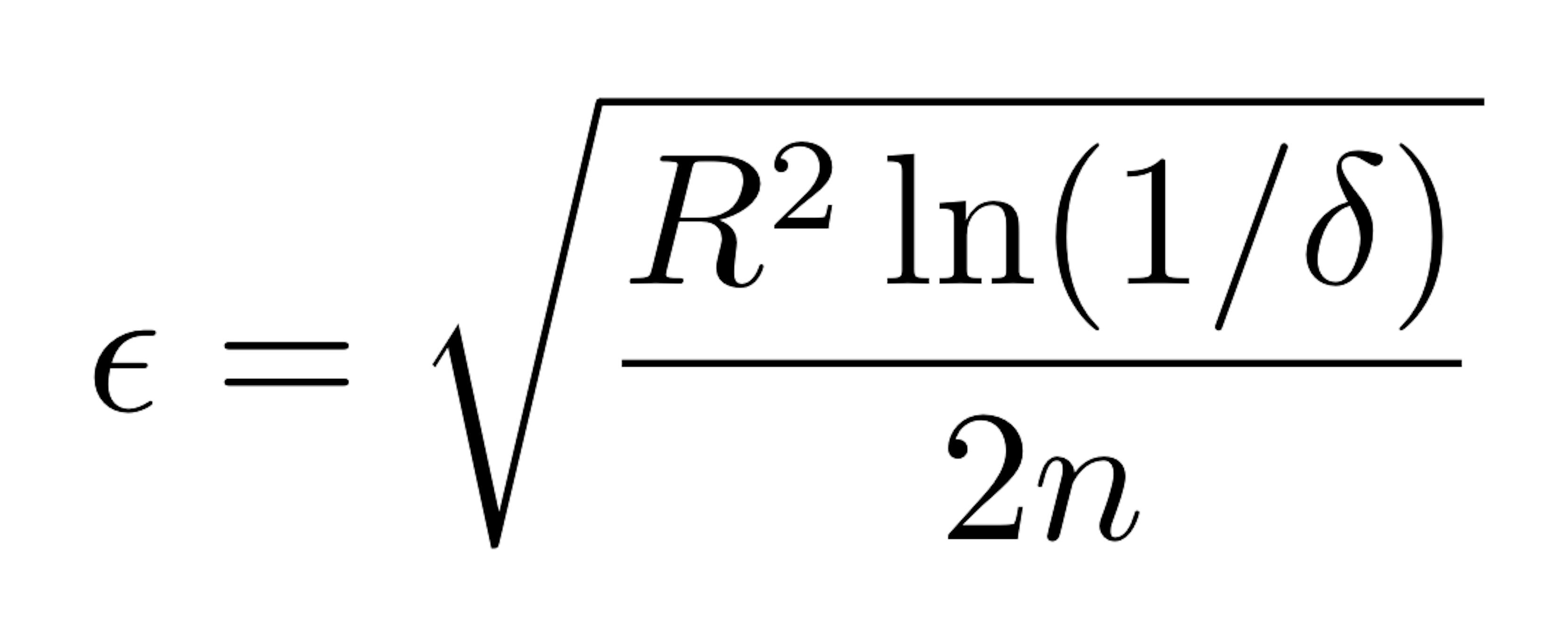
Here R is the range of the independent random variable (e.g. for probability, the range is one, and for information gain the range is log c, where c is the number of classes), n is the total number of examples seen, and delta is the probability bound we specify. The Hoeffding Bound states that the chosen attribute at a specific node, after seeing n number of examples, will be the same attribute as if the algorithm has seen an infinite number of examples, with probability 1 − δ. 

You can see the procedure of the Hoeffding tree on paper but put simply, it's as follows:

1. Initialization. The tree starts with a single root node that eventually branches into a full decision tree.

2. Incremental update. As each new data instance arrives, it's used to update the sufficient statistics for each node in the tree.

3. Split decision. When enough statistics have been gathered at a node, the Hoeffding bound is computed to determine whether a split is warranted.

4. Node splitting. If the Hoeffding bound criterion is met (e.g. information gain exceeds the bound), the node is split using the best attribute. Otherwise, the algorithm continues to collect more data.

EFDT

Copy link

EFDT builds upon the principles of VFDT but incorporates additional mechanisms to enhance its flexibility and adaptiveness. EFDT addresses some of VFDT's limitations by integrating a dynamic structure that can adaptively grow and prune itself in response to changes in the underlying data stream.

EFDT introduces two major improvements over VFDT:

1. Adaptive splitting. While VFDT splits nodes based only on the initial decision, EFDT allows nodes to be revisited and reevaluated continually, providing an opportunity to make better splitting decisions as more data becomes available. This adaptation helps EFDT perform better in environments where data distributions may shift over time. Additionally, this works as a sort of feature selection, and EFDT may work better in conditions of correlating or non-informative features.

2. Pruning mechanism. EFDT includes a pruning mechanism to remove suboptimal branches of the tree, which helps prevent overfitting. The pruning strategy is typically based on statistical measures that identify and eliminate branches that contribute minimally to the overall predictive accuracy.

In fact, these optimizations slow down the algorithm's operation time, which in my opinion, contradicts the title "Extremely." But that's how it turned out.

VFDT vs. EFDT

Copy link

Despite some similarities, VFDT and EFDT differ primarily in their adaptability and complexity of operations:

• EFDT is more adaptive than VFDT. EFDT continually reviews and improves its splits, better adapting to changes in data flows, which is critical in the event of data drift.
• VFDT does not incorporate a pruning mechanism, which can lead to excessively large trees when dealing with noisy data. EFDT's pruning capabilities help maintain a more compact and generalizable tree structure.
• EFDT tends to be more computationally intensive. This means it might be slower than VFDT in scenarios where the data stream is exceedingly fast, but it generally achieves higher accuracy.

So, although VFDT seems to be losing to EFDT in certain aspects, in many services, especially those related to Internet traffic, VFDT's speed can be a decisive advantage for using it. Therefore, consider your requirements and data features when choosing an algorithm. As always.

Code examples (and a little investigation)

Copy link

Let's look at some real implementations. I'll use the skmultiflow library, which provides a wide range of incremental algorithms. I'll start with the MNIST dataset to demonstrate that everything works.

from sklearn.datasets import load_digits
from sklearn.model_selection import train_test_split
from sklearn.metrics import f1_score

from skmultiflow.trees import HoeffdingTreeClassifier, ExtremelyFastDecisionTreeClassifier
import numpy as np
from tqdm.auto import tqdm
import matplotlib.pyplot as plt

df = load_digits()
df = load_digits()
X, y = df['data'], df['target']
X_train, X_test, y_train, y_test = train_test_split(X, y, test_size=0.2)

HoeffdingTreeClassifier is a regular VFDT. Let's check if it works:

ht = HoeffdingTreeClassifier(split_criterion='gini')
ht.fit(X_train, y_train)
print(f1_score(y_test, ht.predict(X_test), average='weighted'))
>>>> 0.9062518655306745

On my laptop, it took about 3 seconds. It would be much longer if we were training any classic decision tree or even random forest, but we're here to work with streaming data, so let's emulate that.

ht = HoeffdingTreeClassifier(split_criterion='gini')
ht_scores = []
for x, y in tqdm(zip(X_train, y_train), total=len(X_train)):
    ht_scores.append(f1_score(y_test, ht.predict(X_test), average='weighted'))
    ht.partial_fit(x.reshape(1, -1), [y])
>>>> 100% 1437/1437 [15:30<00:00, 1.56it/s]

In my opinion, 15 minutes is a lot, but let's look at the graph of the change in the f1-score during the training.

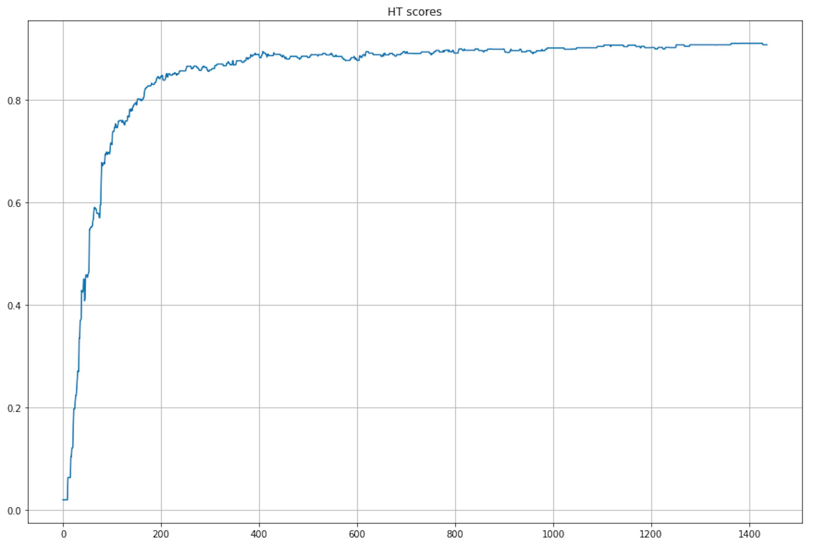
We see that our tree has achieved near-optimal performance on data row 400. This is good news, but the training is still taking too long, obviously. Let's do the same with EFDT.

efdt = ExtremelyFastDecisionTreeClassifier(split_criterion='gini')
efdt_scores = []
for x, y in tqdm(zip(X_train, y_train), total=len(X_train)):
    efdt_scores.append(f1_score(y_test, efdt.predict(X_test), average='weighted'))
    efdt.partial_fit(x.reshape(1, -1), [y])
>>>> 100% 1437/1437 [15:23<00:00, 1.55it/s]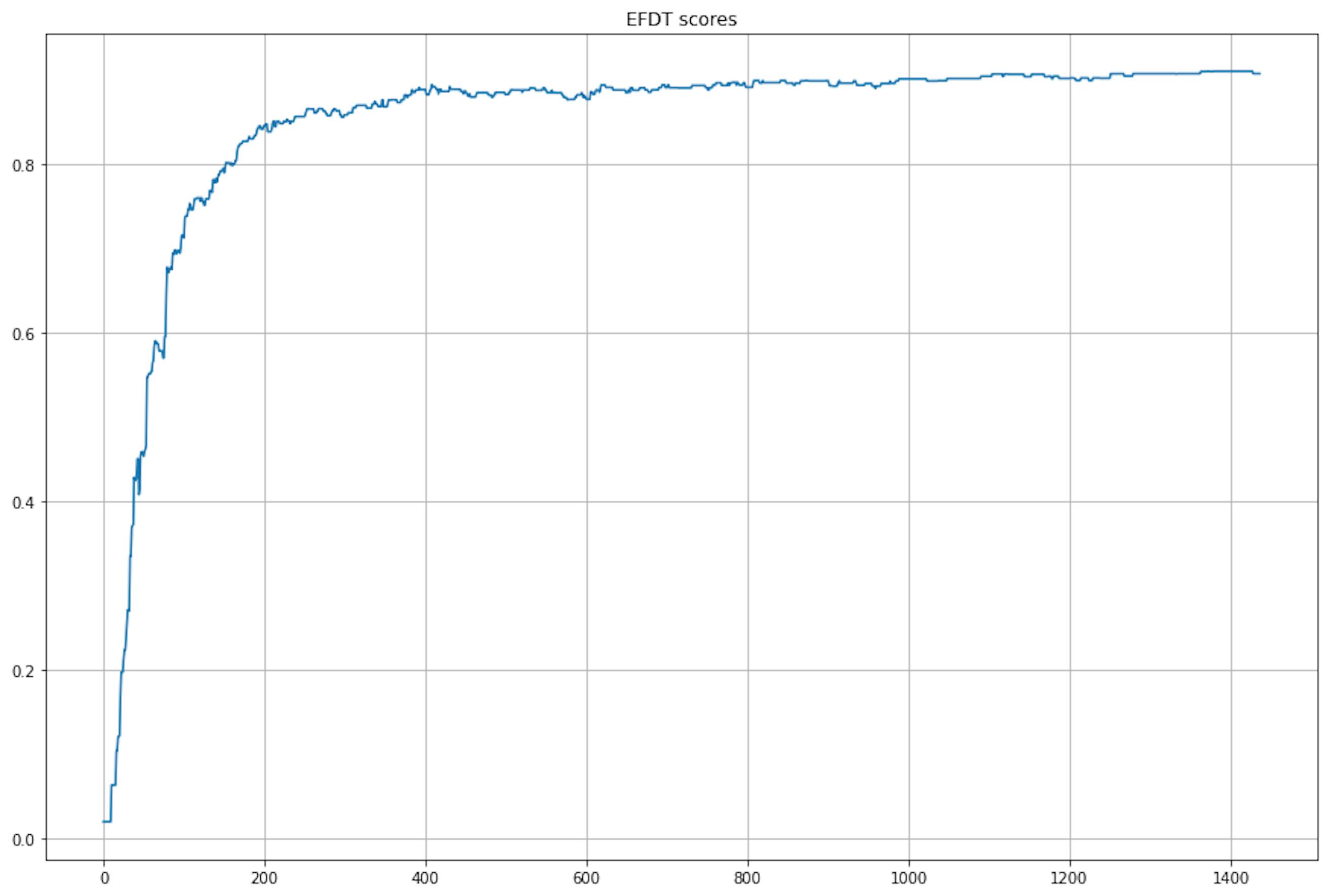

It took the same amount of time, and even the graphs of the change in the score look suspiciously similar.

print(ht_scores == efdt_scores)
>>>> True

And they are similar… So, my first thought was that there was a bug in my code, and the second thought was that there were bugs in the library. But everything was fine. Then, I remembered that MNIST is quite an optimized dataset and good from all points of view. So I decided to test the algorithms on the worst dataset with correlated features and data drift.

Below, I'll measure the accuracy score on the entire training dataset up to the example on which the model is currently being trained. This will be okay for testing.

from sklearn.datasets import make_classification
X, y = make_classification(n_samples=1000, n_features=20, n_informative=2, n_redundant=6, shuffle=True)
shift = np.random.random_sample(20)
X[500:] += shift
ht = HoeffdingTreeClassifier(split_criterion='gini')
ht_scores = []
for i in range(len(X)):
    ht_scores.append(ht.score(X[:i], y[:i]))
    ht.partial_fit(X[i].reshape(1, -1), [y[i]])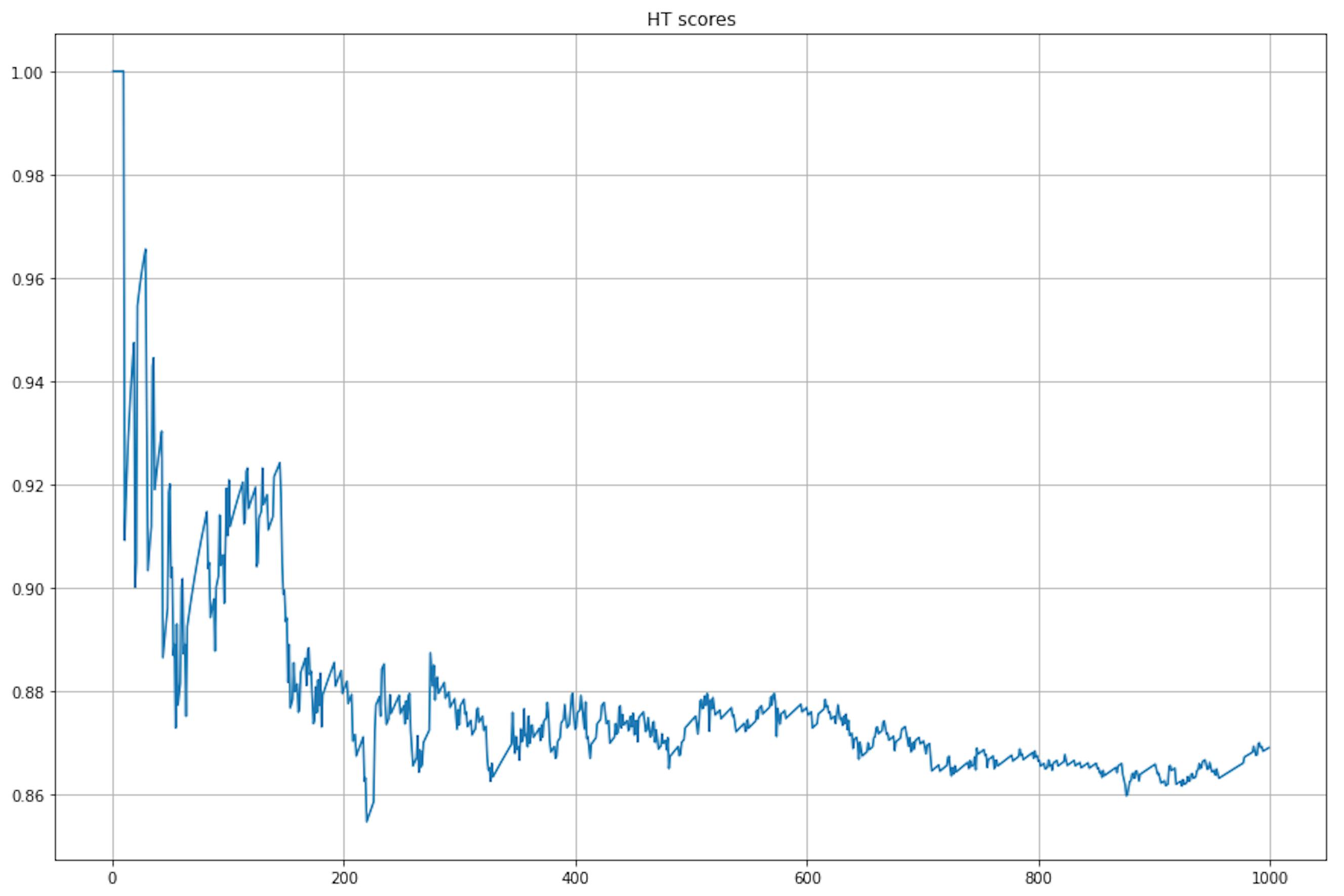

We see that the model cannot fit the dataset (due to correlated and redundant features), and when data drift appears, the scores continue to drop.

efdt = ExtremelyFastDecisionTreeClassifier(split_criterion='gini')
efdt_scores = []
for i in range(len(X)):
    efdt_scores.append(ht.score(X[:i], y[:i]))
    efdt.partial_fit(X[i].reshape(1, -1), [y[i]])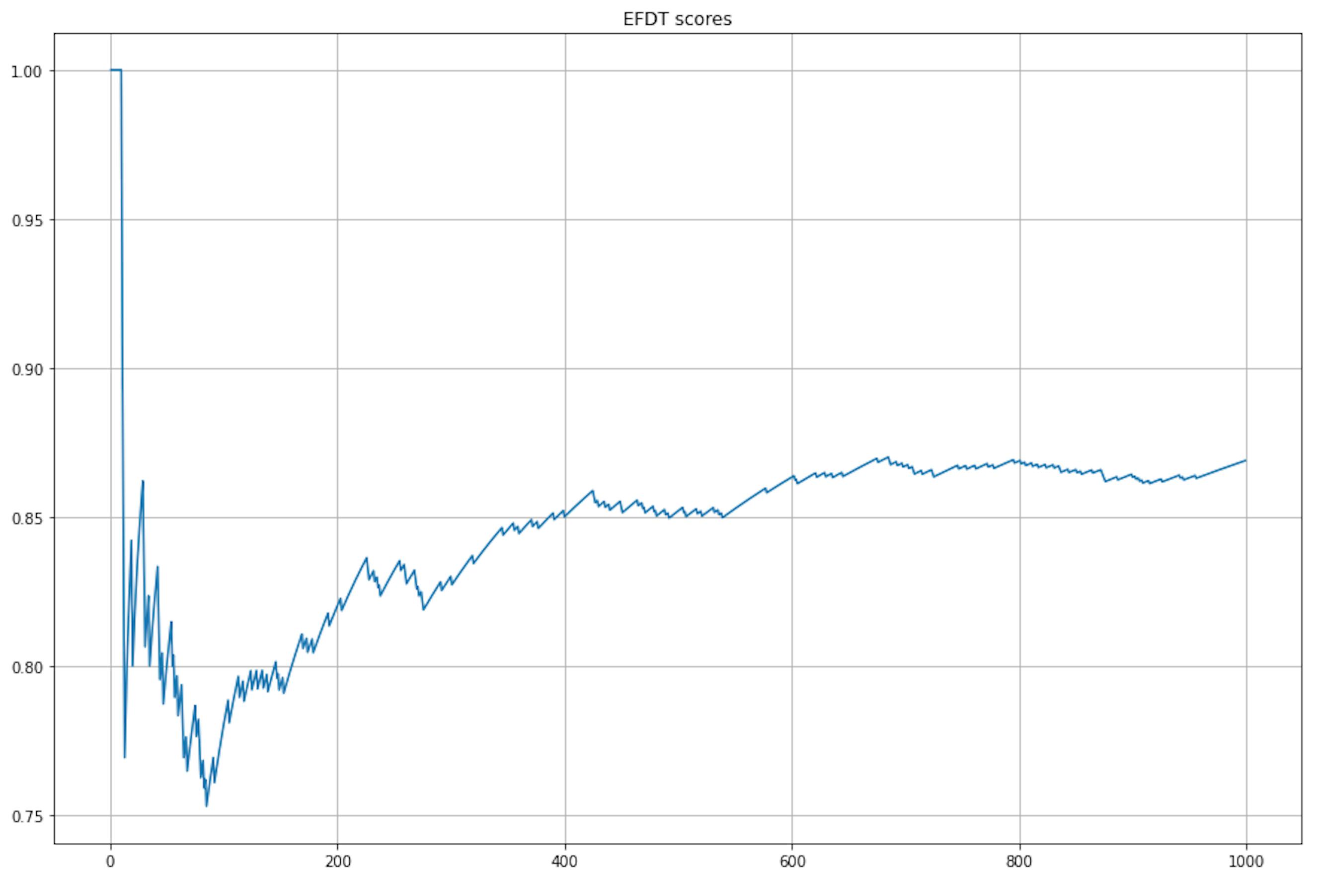

On the other hand, although maximum quality is achieved later, EFDT handled the complex data and continued to improve quality even after data drift.

Alternatives

Copy link

Even though the algorithms work as expected from a learning perspective, the speed is too slow. When we implemented VFDT in the service, this was critical, and I started looking for alternatives and found this implementation: https://github.com/doubleplusplus/incremental_decision_tree-CART-Random_Forest

With all due respect to the developer, the code requires refactoring (which we did), but the code doesn't contain any additional optimizations. This is a pure paper algorithm; therefore, it's very fast.

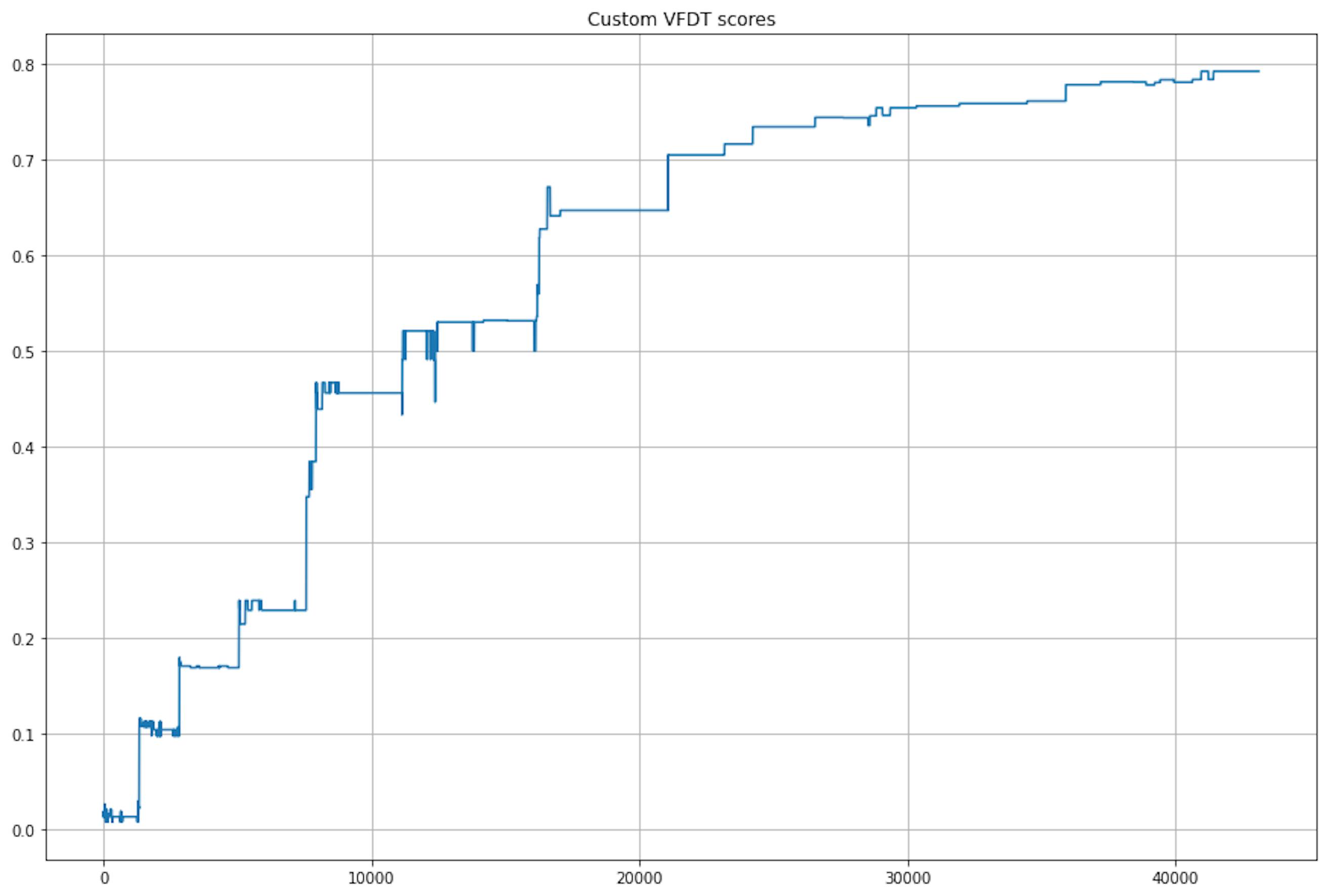
Of course, it has its limitations. For example, in order to get a result comparable in quality to MNIST, I had to run the entire dataset 30 times (but even then, it took 5 times less time than the model from skmultiflow):

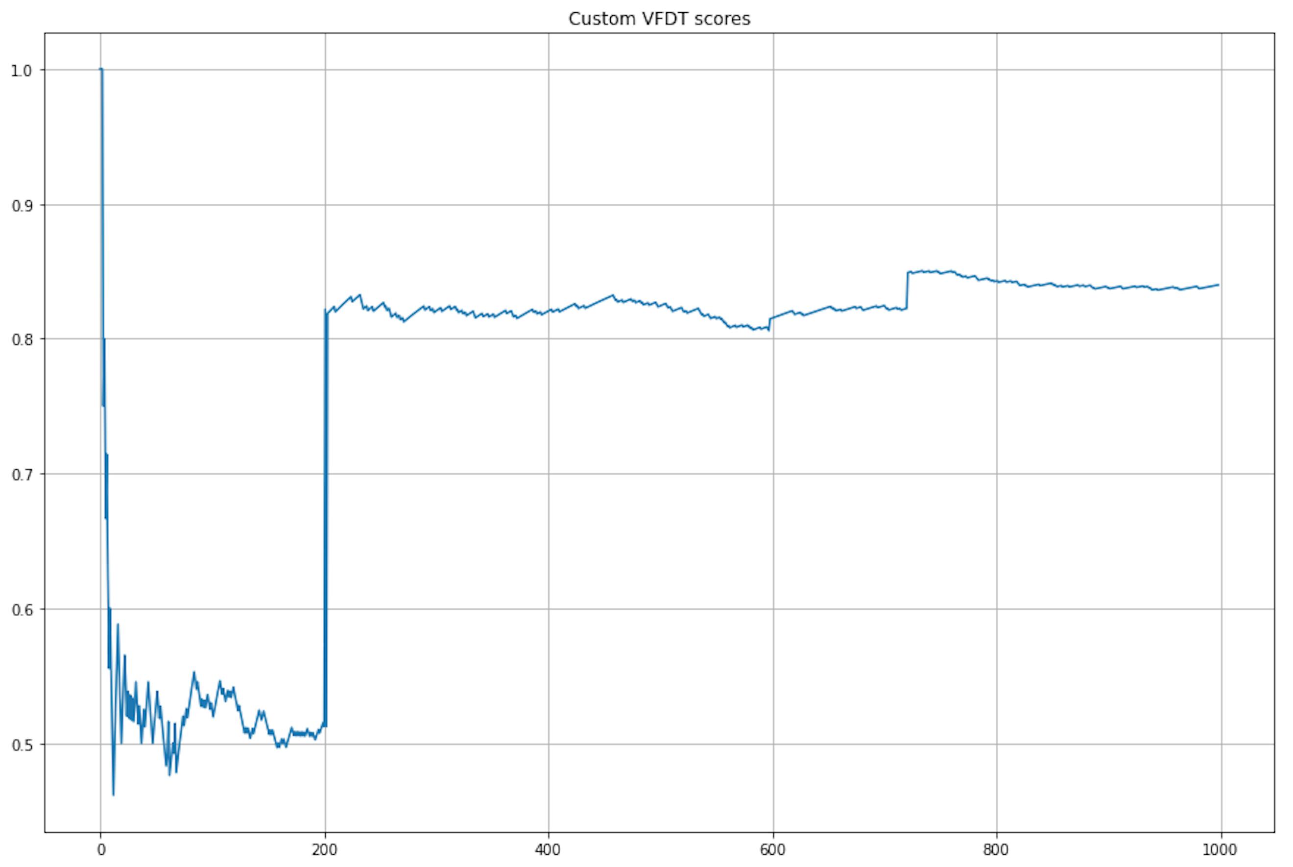
But the model processed the artificial dataset in one second and even displayed high quality:

Conclusion

Copy link

VFDT and EFDT represent significant advancements in decision tree algorithms for streaming data. VFDT offers a balance of speed and simplicity, making it ideal for environments with stable data streams. EFDT, with its adaptive splitting and pruning mechanisms, provides greater adaptability and accuracy, suitable for more dynamic and noisy data environments.

Understanding your application's specific requirements and the nature of your data stream will guide you in selecting the most appropriate algorithm.