Roman Panarin ML Engineer

Created: Jan 15, 2024
Updated: Jan 15, 2024

[Write-up: Basic Data Augmentation Method Applied to Time Series]

Time series are sequences of data points organized over time and are important in a variety of fields including economics, finance, climate science, health, and many others. Analyzing and forecasting time series can provide valuable insights and inform decision making. One of the key obstacles to effective time series analysis is data limitations, which can negatively impact the performance and accuracy of predictive models.

Data augmentation is a set of techniques that are used to increase the size of a dataset by adding modified copies of existing data or creating synthetic data from existing samples. In the context of time series, augmentation can help improve the generalizability of machine learning models by providing them with more diverse examples to train on and thus reducing the risk of overfitting.

In the article, we will review and systematize some augmentation techniques that are applied to time series, study their impact on improving machine learning models and review practical use cases of augmentation in various applications, as well as identify the strengths and weaknesses of each technique.

# Importing libraries

import numpy as np
import random
import matplotlib.pyplot as plt
from scipy.interpolate import CubicSpline

0. Basic definitions

A time series looks as follows:

$X = {x_{0}, x_{1}, . . ., x_{t - 1}, x_{t}, . . . x_{n}}$

where $x_{t}$ - the measurement of some quantity at time $t$ . Sometimes $x_{t}$ represents multiple measurements such as data from a 6-axis accelerometer.

"""
Generating dataset
"""

def bouncing_ball_series(time_steps, initial_height, damping_factor, bounce_frequency):
    """
    Generates a time series that simulates the bounces of a bouncing ball.

    :param time_steps: Number of time steps (data points).
    :param initial_height: Initial bounce height.
    :param damping_factor: Height attenuation coefficient.
    :param bounce_frequency: Bounce frequency (number of bounces per time).
    :return: NumPy array representing the time series.
    """
    # Generate a time array
    time = np.arange(0, time_steps)

    # Function that simulates strikes (sine trimmed to zero and positive values)
    bounces = np.clip(np.sin(bounce_frequency * np.pi * time), 0, None)

    # Exponential decay over time
    damping = np.exp(-damping_factor * time)

    # Series of bounces taking into account attenuation
    series = initial_height * bounces * damping

    return series

# Parameters for generating time series
time_steps = 200          # Number of data points
initial_height = 5.0       # Initial height
damping_factor = 0.03      # Attenuation coefficient
bounce_frequency = 0.1     # Bounce frequency

# Generation of time series
time_series_data = bouncing_ball_series(time_steps, initial_height, damping_factor, bounce_frequency)

# Generation of time series
plt.plot(time_series_data)
plt.title('Pseudo Bouncing Ball Time Series')
plt.xlabel('Time Steps')
plt.ylabel('Height')
plt.show()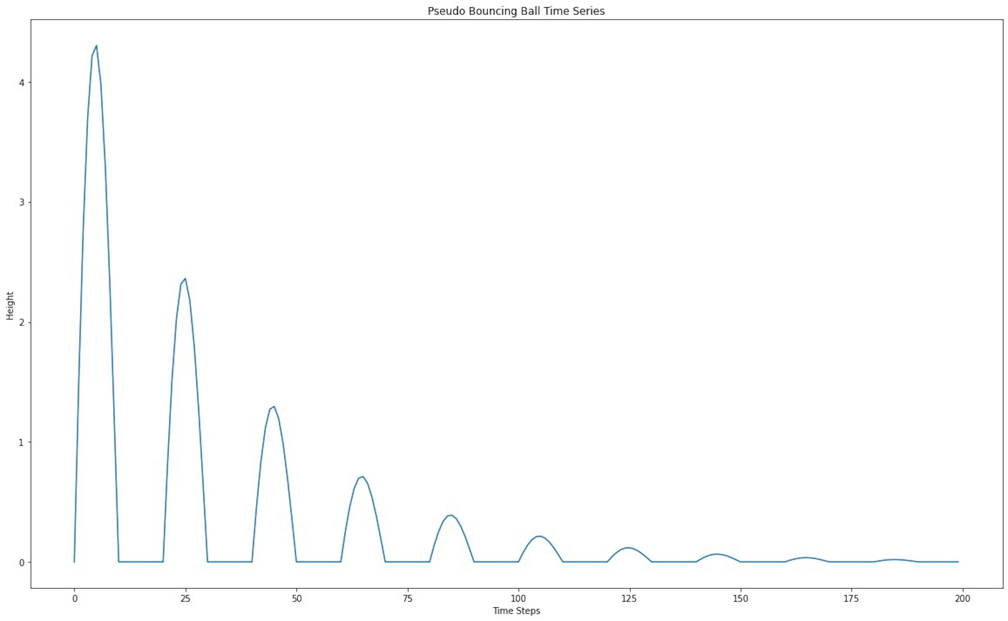

1. Jittering / Gaussian noise

Jittering is a technique for improving time series data by adding random noise to the original signals. This technique improves the robustness and generalizability of machine learning models by simulating small changes in real-world conditions. To augment a time series, you can add Gaussian noise with zero mean and specified variance to each value of the series. This makes the algorithm more tolerant to small deviations and helps prevent overtraining. The mean and standard deviation of this noise determine the amplitude and shape of the deformation, so they are different for each specific application. In terms of mathematical formulation, we perform the following transformation:

$X' = x_{0} + ϵ_{1}, x_{1} + ϵ_{2}, . . ., x_{t} + ϵ_{t}, x_{n} + ϵ_{n}$

where $ϵ \sim N (0, σ^{2})$ - denotes the noise added to each value of the time series.

Gaussian noise is the most popular option, but not the only one. Depending on the task, complex transformations can be used: sawtooth noise, step noise or sloping trend noise.

The technique of adding noise must be adapted to each case because there are cases, such as in this paper, where jitter effects lead to negative learning. In this study, the information used as time series data was taken from a wearable sensor that recorded 58 seconds at 62.5 Hz, which were later resampled to 120 Hz per sample.

def add_gaussian_noise(time_series, mean=0.0, stddev=1.0):
    """
    Adds Gaussian noise to a time series.

     Options:
     time_series (array-like): A time series to which noise is added.
     mean (float): The average value of the noise. Default is 0.0.
     stddev (float): Standard deviation of noise. Default is 1.0.

     Returns:
     noisy_series (np.array): Time series with added noise.
     """
     # Gaussian noise generation
    noise = np.random.normal(mean, stddev, len(time_series))

    # Adding noise to the original time series
    noisy_series = time_series + noise

    return noisy_series

augmented_time_series_data = add_gaussian_noise(time_series_data, mean=0.0, stddev=0.05)

plt.figure(figsize=(20, 12))

plt.subplot(1,2,1)
plt.title("Original Data")
plt.plot(time_series_data)

plt.subplot(1,2,2)
plt.title("Augmented Data")
plt.plot(augmented_time_series_data)
[<matplotlib.lines.Line2D at 0x13e168f40>]

Pros

Expanding the training dataset. The use of noise augmentation increases the number of training examples, helping the model to improve its understanding of time series structure and cope with the overtraining problem

Modeling real-world conditions. Real-world data often contains noise, so noise augmentation can help the model better adapt to such conditions and predict real-world scenarios.

Increasing the robustness of the model. Adding noise enhances the generalizability of the model, making it more robust to small changes in the data, which is especially important in time series forecasting.

Cons

Increasing the complexity of model interpretation. Adding noise can make it more difficult to understand how the model uses the data for forecasting, especially if important time series properties are "lost" among the noise.

The need for fine tuning. Selecting the optimal noise level that will be useful for augmentation can require considerable effort and time. Too much noise can harm the model, and too little noise may not provide the expected benefit.

Risk of signal warping. If noise is added inaccurately, it can distort important time series characteristics such as trends, seasonality and cyclical components, negatively affecting the model's ability to make accurate predictions.

2. Time slicing window

Related to the augmentation method in computer vision, the cropping method (time slicing window) has the disadvantage of cutting off important features that are occluded in the temporal sequence.

The method works as follows:

$X' = {x_{ϕ}, . . ., x_{t}, . . ., x_{ϕ + w i d t h}}$

where $w i d t h$ - is the window width, which determines the size of the sliced part of the time series. Value $ϕ$ - defines the starting point from which the cut is performed.

plt.figure(figsize=(20, 12))

plt.subplot(1,2,1)
plt.title("Original Data")
plt.plot(time_series_data[:])
plt.axvspan(60, 110, facecolor='y', alpha=0.5);

plt.subplot(1,2,2)
plt.title("Augmented Data")
plt.plot(np.concatenate((time_series_data[0:60], time_series_data[110:-1])))
[<matplotlib.lines.Line2D at 0x13de1fa60>]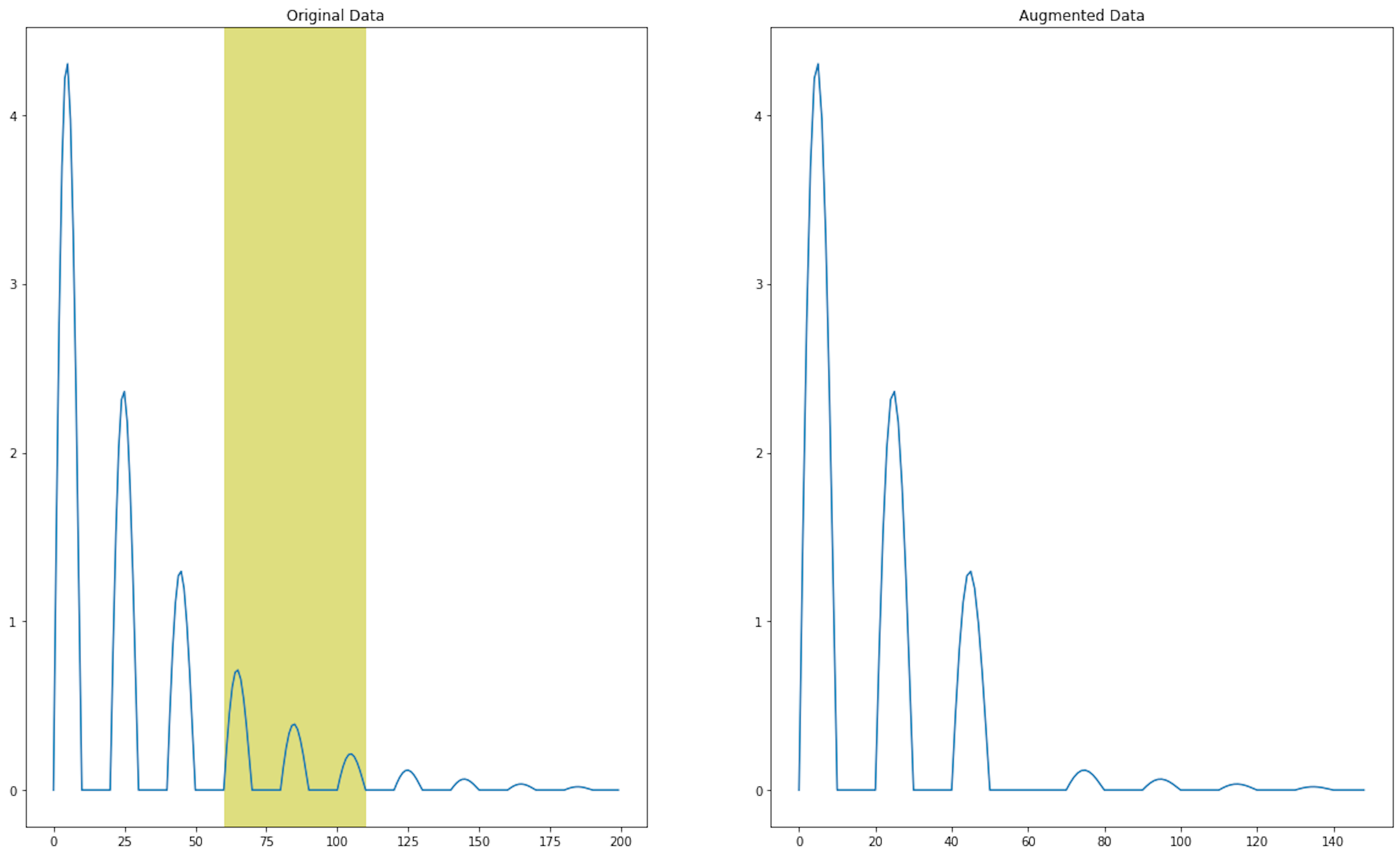

Pros

Increasing the training dataset. Cropping allows a significant increase in the number of available training examples without the need to collect new data. This can be particularly useful when the original time series is limited or expensive to obtain.

Preventing overfitting. Using different segments of a time series as independent samples can help create a more robust model that generalizes better and is less prone to overfitting on noise or irrelevant features of the original time series.

Increased invariance to time scale. Training on truncated time series can make the model more invariant to time scale, which means improving the model's ability to recognize patterns in the data, regardless of their duration or initial time position in the original series.

Cons

Loss of information. Cropping can lead to the loss of important information contained in the relationships between distant parts of a time series. This is especially true for processes where long-term dependencies are critical to understanding and predicting the behavior of the time series

Risk of inducing artificial bias. Although data augmentation should increase the generalizability of the model, improper application of cropping can lead to the introducing of artificial bias in the training set if, for example, some important events or patterns are always cropped and not represented in the augmented data.

The complexity of selecting a window size. Choosing an appropriate time window size for augmentation can be a non-trivial task. A window that is too large can cut out too much information, and a window that is too small can change the original data too little, making augmentation less efficient. Finding a balance that optimizes model performance can require a lot of experimentation and tuning.

3. Scaling

A scaling procedure is a change in the amplitude of the value of a certain dimension of a time series. The basic idea of this approach is the transformation of the range of values, but while preserving the shape of the time series. Mathematical formulation of scaling is the following:

$X' = {α * x_{0}, . . ., α * x_{t}, . . ., α * x_{n}}$

where $α > 0$ - is the scaling coefficient. In practice this coefficient is most often taken as a value from the Gaussian distribution with mean value = 1 and variance $σ - N (0, σ^{2})$ .

def add_scaling(time_series, scale_factor):
    """
    Scales a time series by multiplying each element by scale_factor.

    :param time_series: numpy array, time series to be scaled
    :param scale_factor: the number by which all elements of the series will be multiplied
    :return: numpy array, scaled time series
    """
    scaled_time_series = time_series * scale_factor
    return scaled_time_series

scale_factor = 0.48

augmented_time_series_data = add_scaling(time_series_data, scale_factor)
plt.figure(figsize=(20, 12))

plt.subplot(1,2,1)
plt.title("Original Data")
plt.plot(time_series_data[:])

plt.subplot(1,2,2)
plt.title("Augmented Data")
plt.plot(augmented_time_series_data, label="Augmented data")
plt.plot(time_series_data[:], label="Origin Data")
plt.legend()
<matplotlib.legend.Legend at 0x13e4feaa0>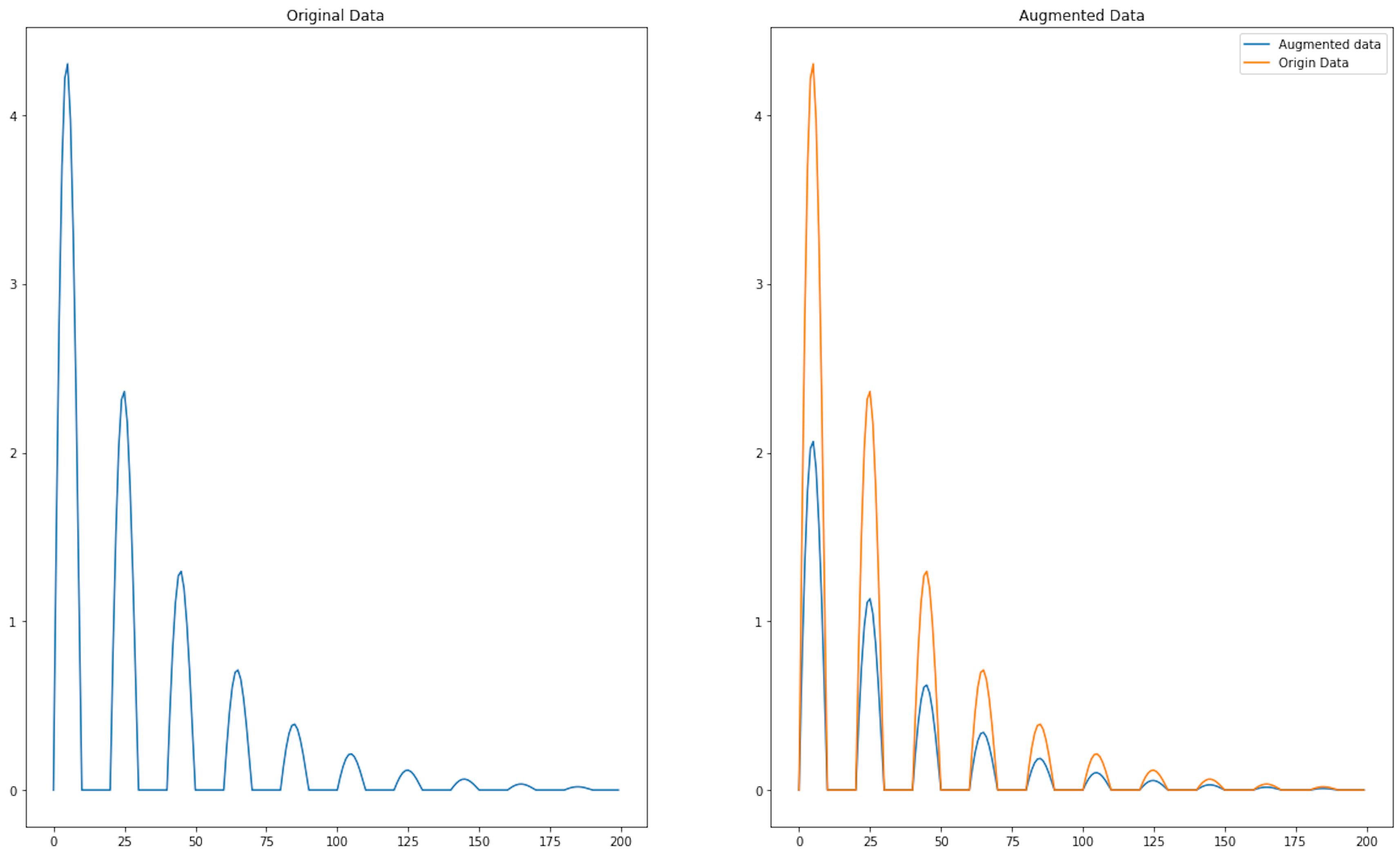

Pros

Improving the generalizability of the model. Scaling allows you to create modified versions of the original time series at different scales. This can help machine learning algorithms to better generalize results and improve the model's robustness to changes in the scale of the input data.

Increased robustness to variations in amplitude. Scaling augments the data so that the model learns to be robust to changes in signal amplitude, which is important, for example, in financial forecasting or health monitoring, where amplitude can change due to external factors.

Cons

Potential loss of important information. Scaling can distort important time series properties such as trends, seasonality and cyclicality. This can lead to the creation of unrepresentative data samples that may mislead the model.

Risk of overfitting on augmented data. If scaling is applied carelessly, there is a risk that the model will be overfitted with artificially created patterns, impairing its predictive ability on new, non-augmented data.

3.1. Magnitude Warping

Identify the warping locations. For this purpose, we define a set of steps $u = u_{1}, u_{2}, . . ., u_{i}$ - at which the scaling is performed. The values for these nodes are generated using a normal distribution.
Next, for each point between the nodes, the scaling amplitudes are determined using cubic spline interpolation of the nodes $S (x)$

The formal mathematical formulation is as follows: $x' (a) = {a_{1} * x_{1}, . . ., a_{t} * x_{t}, . . ., a_{n} * x_{n}}$ , where $a = a_{1}, . . ., a_{i} = S (x)$ .

This technique was used in paper where the data was captured from a wearable device to detect if a patient suffers from Parkinson’s disease.

One of the options for magnitude warping is frequency warping, an algorithm often used in speech processing. The most popular version in speech recognition is Vocal Tract Length Perturbation, which can be applied in a deterministic way or stochastically within a range. In particular, this technique was used in article where a dataset of human conversation sampled at 8 KHz was used.

def magnitude_warping(time_series, num_knots=4, warp_std_dev=0.2):
    """
    Applies magnitude warping to a time series using cubic splines.

    :param time_series: np.array, time series to distort
    :param num_knots: int, number of control points for splines
    :param warp_std_dev: float, standard deviation for distorting the values of control points
    :return: np.array, distorted time series
    """
    # Generating random spline knots within a time series
    knot_positions = np.linspace(0, len(time_series) - 1, num=num_knots)
    knot_values = 1 + np.random.normal(0, warp_std_dev, num_knots)

    # Creating a Cubic Spline Function Through Knots
    spline = CubicSpline(knot_positions, knot_values)

    # Generating time indexes for a time series
    time_indexes = np.arange(len(time_series))

    # Applying distortion to a time series
    warped_time_series = time_series * spline(time_indexes)

    return warped_time_series


augmented_time_series_data = magnitude_warping(time_series_data, num_knots=5, warp_std_dev=0.45)
plt.figure(figsize=(20, 12))

plt.subplot(1,2,1)
plt.title("Original Data")
plt.plot(time_series_data[:])

plt.subplot(1,2,2)
plt.title("Augmented Data")
plt.plot(augmented_time_series_data, label="Augmented data")
plt.plot(time_series_data[:], label="Origin Data")
plt.legend()
<matplotlib.legend.Legend at 0x141910520>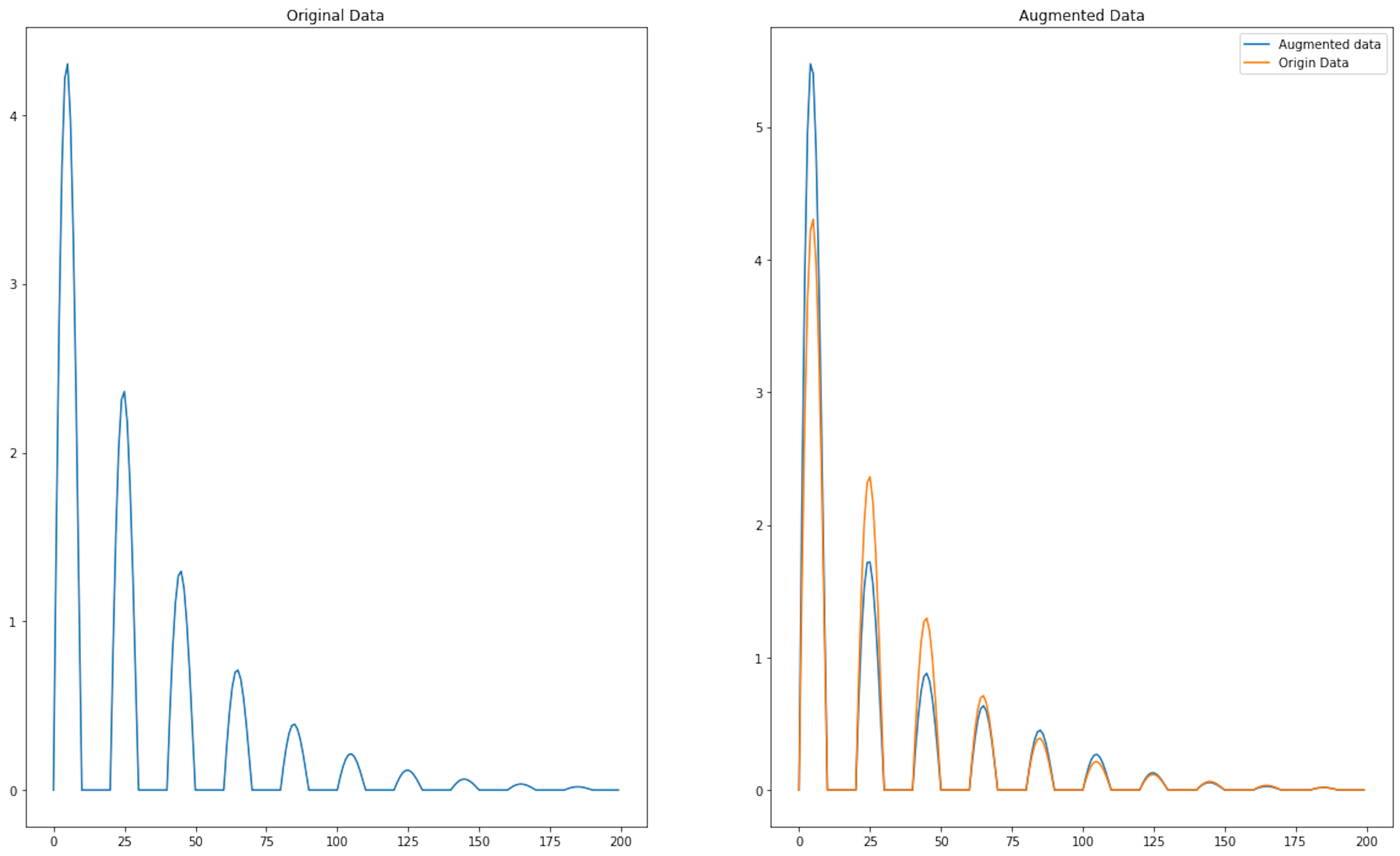

Pros

No Need for Additional Data. Magnitude Warping can create new datasets without the need to collect new real-world data, saving time and resources.

Customizable Augmentation. The algorithm's parameters can be adjusted to control the amount and type of warping applied to the time series, allowing for flexibility in creating tailored augmentations for the task at hand.

Simplicity and Speed. Magnitude Warping is generally simple to implement and fast to execute, meaning it can be easily integrated into the data preprocessing pipeline.

Cons

Limited to Magnitude Changes. Magnitude Warping primarily focuses on varying the magnitude of data points, and might not capture other important characteristics of time series data, such as frequency or time-dependent patterns.

No New Information. Since the augmented data are derived from the original dataset, no new information is added to the model. This can be a limitation if the original data doesn't capture all the nuances of the problem space.

Ineffectiveness For Certain Applications. Magnitude Warping is not suitable for all types of time series data. For example, with highly structured or periodic data, warping may distort the underlying patterns and render the augmented data less useful.

3.2. Time Warping

Another advanced time series scaling technique is time warping. This algorithm is similar to magnitude warping, but instead of changing the amplitude of the signal at each step, time warping stretches and compresses the signal. With this augmentation, we make our model more robust to the sampling of the signal.

def time_warping(time_series, num_operations=10, warp_factor=0.2):
    """
    Applying time warping to a time series.

    :param time_series: Time series, numpy array.
    :param num_operations: Number of insert/delete operations.
    :param warp_factor: Warp factor that determines the impact of operations.
    :return: Distorted time series.
    """
    warped_series = time_series.copy()
    for _ in range(num_operations):
        operation_type = random.choice(["insert", "delete"])
        index = random.randint(1, len(warped_series) - 2)
        if operation_type == "insert":
            # Insert a value by interpolating between two adjacent points
            insertion_value = (warped_series[index - 1] + warped_series[index]) * 0.5
            warp_amount = insertion_value * warp_factor * random.uniform(-1, 1)
            warped_series = np.insert(warped_series, index, insertion_value + warp_amount)
        elif operation_type == "delete":
            # Remove a random point
            warped_series = np.delete(warped_series, index)
        else:
            raise ValueError("Invalid operation type")

    return warped_series

augmented_time_series_data = time_warping(time_series_data, num_operations=20, warp_factor=0.25)
plt.figure(figsize=(20, 12))

plt.subplot(1,2,1)
plt.title("Original Data")
plt.plot(time_series_data[:])

plt.subplot(1,2,2)
plt.title("Augmented Data")
plt.plot(time_series_data[:], label="Origin Data")
plt.plot(augmented_time_series_data, label="Augmented data", linestyle="--")
plt.legend()
<matplotlib.legend.Legend at 0x142339ed0>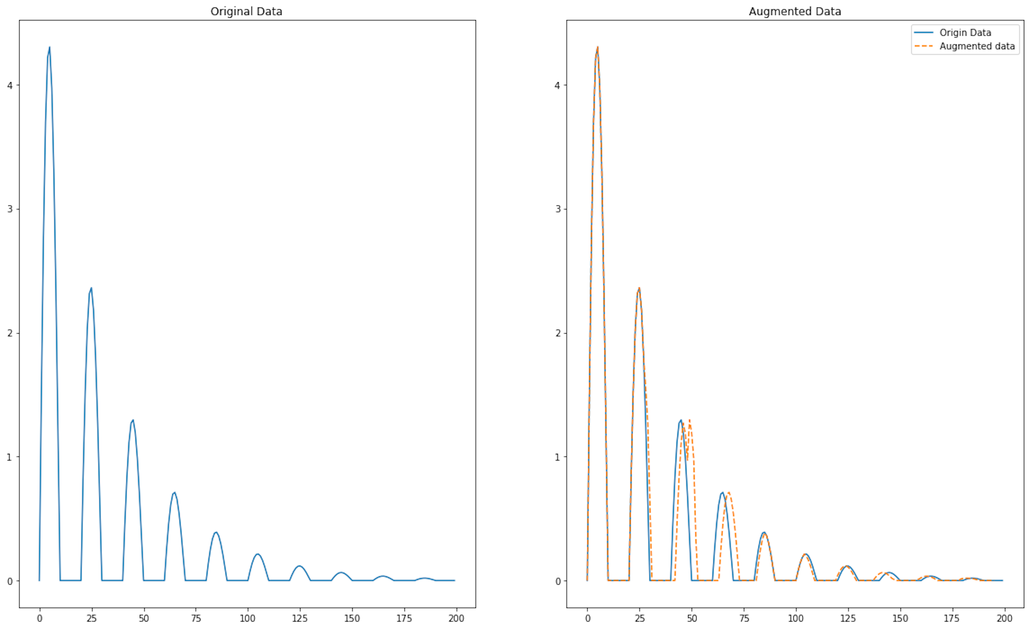

This algorithm has a modification, window warping, described in paper, which defines a slice of the time series data and speeds up or reduces the data processing speed by a factor of 1/2 or 2. The deformation is applied to a certain fragment of the whole sequence, the rest of the signal is not changed.

Pros

Better Invariance. Training with warped time series can help the model to learn invariance to time deformation, which is beneficial when dealing with time-related variances in real-world scenarios.

Efficiency. Time Warping can be computationally efficient compared to other data augmentation methods, especially when applied in a batch-wise manner during the training process.

Customizability. The degree of warping can be controlled, allowing the creation of subtle to significant variations based on the desired augmentation effect.

Cons

Domain-Specific Limits. Not all time series datasets can benefit from time warping similarly. In certain domains, such as medical ECG data, excessive warping might lead to non-physiological patterns that could harm model performance.

Parameter Tuning. Deciding on the optimal parameters for time warping requires experimentation, which can be time-consuming and may require domain expertise to ensure realistic augmentations.

Dependency on Data Quality. Time Warping assumes the underlining quality of the data is good. If the original data contains noise or errors, augmenting it might amplify these issues.

4. Permutation

This algorithm mixes different time slices of the signal. Mathematically, the algorithm looks as follows:

$x' (w) = {x_{i}, . . ., x_{i + w}, . . ., x_{j}, . . ., x_{j + w}, . . ., x_{k}, . . ., x_{k + w}}$

where, i, j, k represent the first slice indexes for each window, so that each index is selected exactly once, and w denotes the window size.

def shuffle_time_slices(time_series, slice_size=1):
    """
    Shuffle different time slices of the provided array.

    Parameters:
    time_series (array-like): An array containing time-series data.
    slice_size (int): The size of each time slice that will be shuffled.

    Returns:
    shuffled_data (array-like): The array with shuffled time slices.
    """

    # Convert to numpy array if not already
    time_series = np.array(time_series)

    if slice_size <= 0 or slice_size > len(time_series):
        raise ValueError("Slice size must be within the range 1 to len(data)")

    num_slices = len(time_series) // slice_size

    # Cut the data into slices
    slices = [time_series[i * slice_size:(i + 1) * slice_size] for i in range(num_slices)]

    # Shuffle the slices
    np.random.shuffle(slices)

    # Concatenate the shuffled slices
    shuffled_data = np.concatenate(slices)

    # Include any leftover data that couldn't form a complete slice
    remainder = len(time_series) % slice_size
    if remainder > 0:
        remainder_data = time_series[-remainder:]
        shuffled_data = np.concatenate([shuffled_data, remainder_data])

    return shuffled_data

augmented_time_series_data = shuffle_time_slices(time_series_data, slice_size=30)
plt.figure(figsize=(20, 12))

plt.subplot(1,2,1)
plt.title("Original Data")
plt.plot(time_series_data[:])

plt.subplot(1,2,2)
plt.title("Augmented Data")
plt.plot(augmented_time_series_data)
plt.legend()
WARNING:matplotlib.legend:No artists with labels found to put in legend.  Note that artists whose label start with an underscore are ignored when legend() is called with no argument.
<matplotlib.legend.Legend at 0x1420bf160>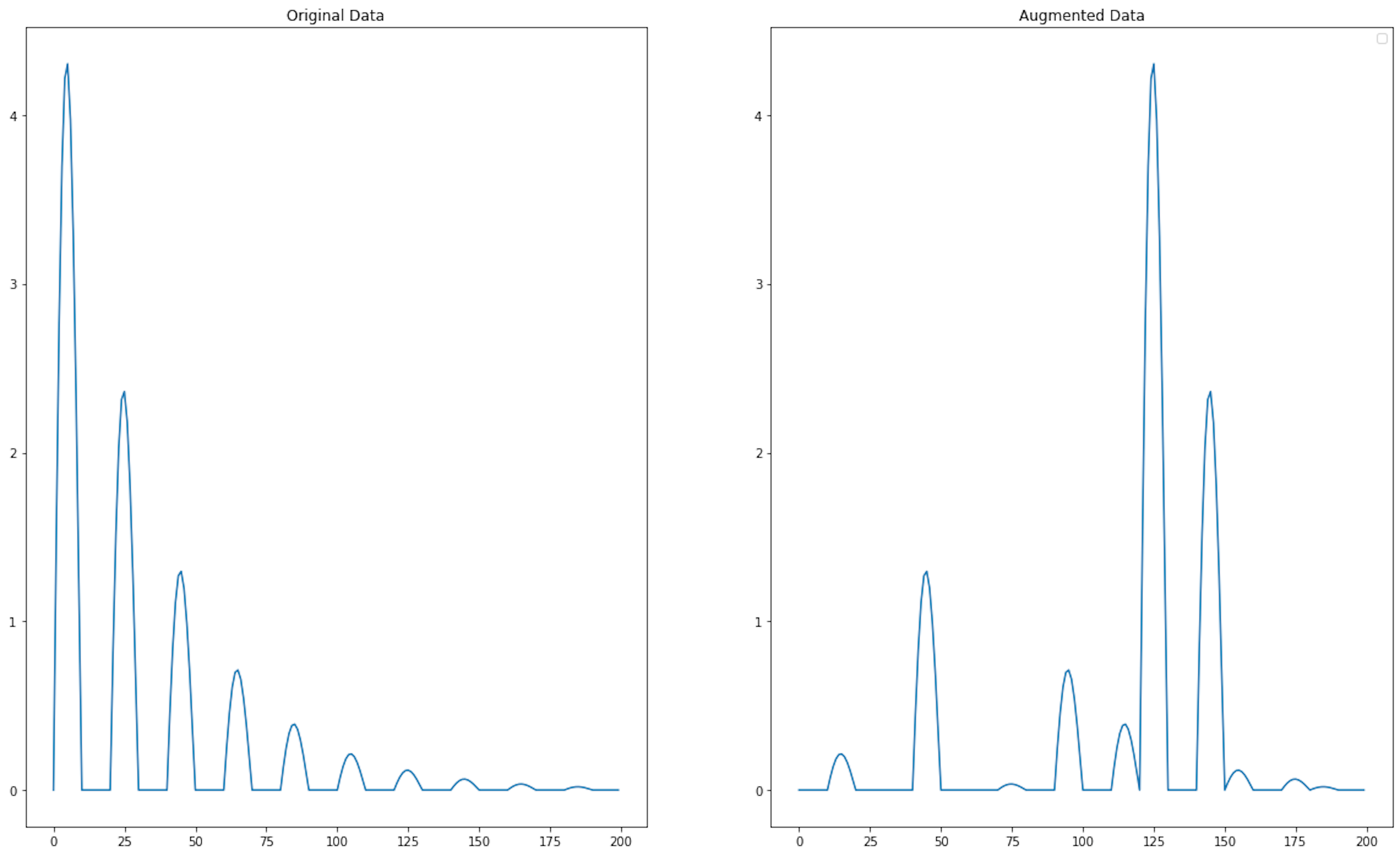

The main problem with using permutation is that it does not preserve temporal dependencies; thus, this may result in invalid samples. But permutation methods can be useful in classification or anomaly detection problems.

Pros

No Additional Domain Knowledge Needed. Permutation is a generic method that doesn't rely on understanding the specific context of the data. It can be applied to any time series regardless of the domain.

Maintained Autocorrelation. When applied carefully, such as by permuting within segments, the algorithm can maintain some level of the original autocorrelation structure of the data, allowing the augmented data to remain realistic.

Cons

Loss of Temporal Structure. Time series data often has important temporal dependencies. Permutation can disrupt these dependencies, leading to synthetic data that no longer represents realistic temporal patterns, which can mislead the model.

Context Ignorance. Time series data often have contextual or seasonal trends (e.g., financial data often have trends and cycles). Permutation can disrupt these trends, making the augmented data less representative of the real-world context.

5. Rotation

Rotation can be applied to multivariate time series by using a rotation matrix with a certain angle. In the case of univariate time series, rotation is accomplished by flipping the data. For multivariate time series, the new sample is defined as follows:

$x' (R) = {R x_{1}, \dots, R x_{t}, \dots, R x_{T}}$

where R — is the rotation matrix used for data augmentation. The rotation angle of $θ$ is chosen randomly from a normal distribution. However, this algorithm is not often applied because rotation of the time series sample can lead to loss of class information.

def rotation(time_series, sigma=1.0):
    """
    Rotates a time series using an angle selected from normal distribution with standard deviation sigma.

    :param time_series: list or np.array, time series for augmentation
    :param sigma: float, standard deviation of the rotation angle in degrees
    :return: np.array, rotated time series
    """
    # Generating the rotation angle from the normal distribution
    angle = np.random.normal(scale=sigma)
    # Convert angle to radians
    angle_rad = np.deg2rad(angle)

    # Creating a rotation matrix
    rotation_matrix = np.array([
        [np.cos(angle_rad), -np.sin(angle_rad)],
        [np.sin(angle_rad), np.cos(angle_rad)]
    ])

    # Let's transform the time series into a two-dimensional array, where each point is a pair (time, value)
    time_indices = np.arange(len(time_series)).reshape(-1, 1)
    values = np.array(time_series).reshape(-1, 1)
    two_dim_points = np.hstack((time_indices, values))

    # Apply the rotation matrix to each point in the time series
    rotated_points = two_dim_points.dot(rotation_matrix)

    # Returning only time series values after rotation
    return rotated_points[:, 1]

augmented_time_series_data = rotation(time_series_data)
plt.figure(figsize=(20, 12))

plt.subplot(1,2,1)
plt.title("Original Data")
plt.plot(time_series_data[:])

plt.subplot(1,2,2)
plt.title("Augmented Data")
plt.plot(augmented_time_series_data)
plt.legend()
WARNING:matplotlib.legend:No artists with labels found to put in legend.  Note that artists whose label start with an underscore are ignored when legend() is called with no argument.
<matplotlib.legend.Legend at 0x142209930>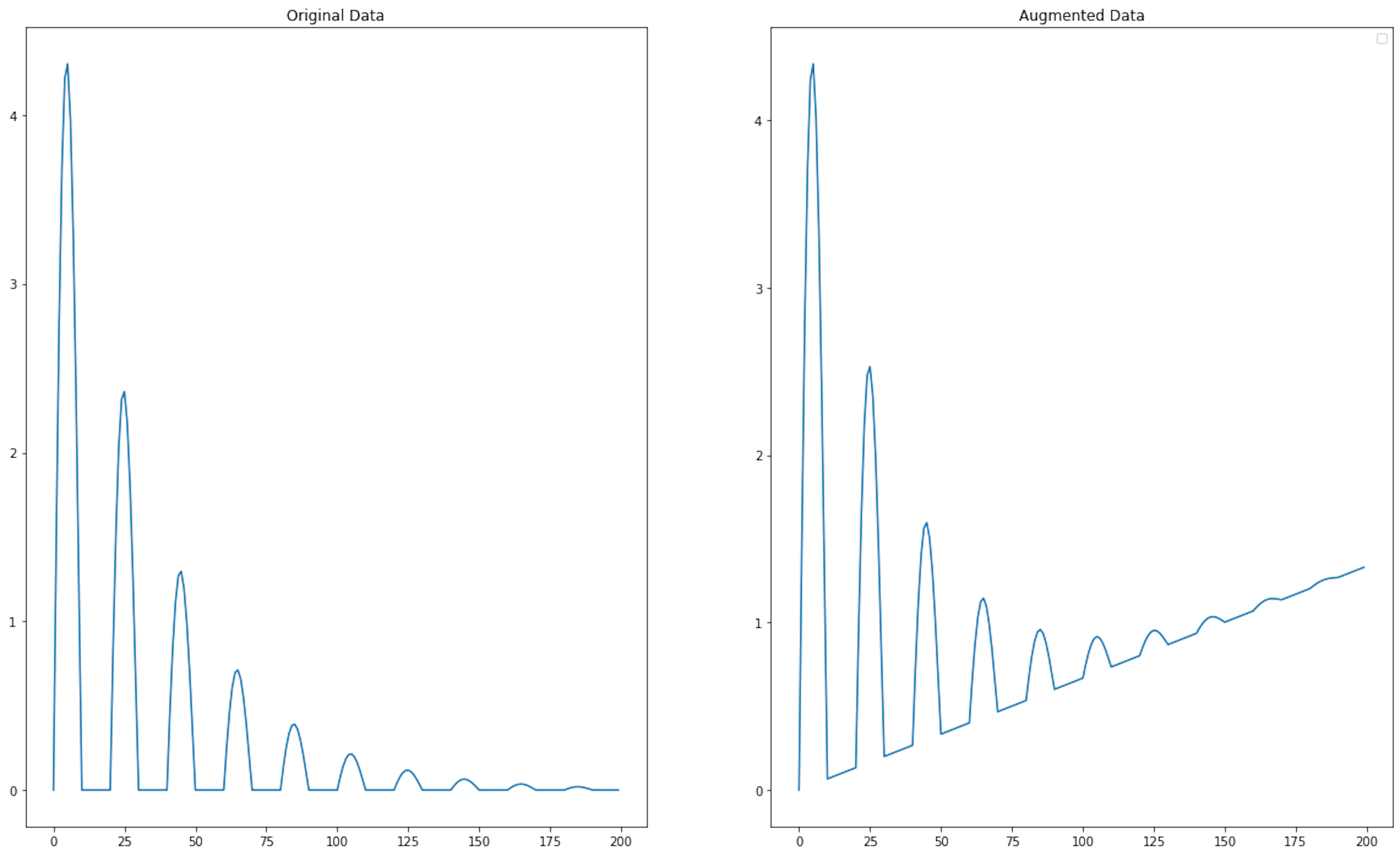

This type of augmentation should be used with caution because it leads to violations of the physical laws on which some of the collected time series data are based.

Pros

Maintains Temporal Dynamics. Unlike some augmentation techniques that may distort the temporal dynamics of the series, rotation keeps the temporal sequence intact, simply rotating the amplitude of the data.

Cons

Risk of Misleading the Model. If the rotation is not representative of natural variations within the dataset, it could mislead the model and contribute to poorer performance on actual data.

Normalization Requirement. For rotation to be effective, the time series data may need to be normalized so that the rotations make sense and do not produce outlier values that could negatively affect the model.

Loss of Meaning. In some contexts, the rotation of a time series might result in data that no longer carries the same meaning, which may be counterproductive to training the model (e.g., negative values in a series representing absolute quantities like stock prices).

6. Channel permutation

Similar to the popular method of data augmentation in computer vision, when rearranging RGB image channels, time series are no exception. However, it should be taken into account that when rearranging the channels, we have to leave the channels themselves unchanged. This method is often practiced for augmenting data from wearable devices, such as a 6-axis accelerometer-gyroscope.

Pros

Variety in Training Data. It provides a way to artificially expand the training dataset, introducing more variety without collecting new data.

Better Exploitation of Inter-Channel Relationships. It can help models better learn the invariance in the inter-channel relationships, which is especially useful when the relative importance or order of channels to the outcome is unknown or variable.

Cons

Potential Loss of Meaningful Information. Channel permutation may break the inherent relationships between channels that are essential for making accurate predictions. In real-world time series applications, the order of channels may carry important contextual or causal information.

Specific to Multivariate Data. Channel permutation is not applicable to univariate time series data.

Parameterization Complexity. Care must be taken in deciding how often and which channels to permute, as too much permutation can make the training data unrealistic, while too little may not provide sufficient augmentation benefits.

Deep learning methods for data augmentation

Very often deep learning methods are used for augmentation of time series data: VAE, GAN and others. They are all implemented in the tsgm library. The essence of these approaches is that we need to train a machine learning model on historical data and teach it to generate new synthetic samples. This is a "black box" method because it is difficult to interpret how the new samples were created.

Reference

Iglesias, G., Talavera, E., González-Prieto, Á. et al. Data Augmentation techniques in time series domain: a survey and taxonomy. Neural Comput & Applic 35, 10123–10145 (2023). https://doi.org/10.1007/s00521-023-08459-3
Um, T.T., Pfister, F.M., Pichler, D., Endo, S., Lang, M., Hirche, S., Fietzek, U., Kuli ́c, D.: Data augmentation of wearable sensor data for parkinson’s disease monitoring using convolutional neural networks. In: Proceedings of the 19th ACM International Conference on Multimodal Interaction, pp. 216–220 (2017)
Cui, X., Goel, V., Kingsbury, B.: Data augmentation for deep neural network acoustic modeling. IEEE/ACM Transactions on Audio, Speech, and Language Processing 23(9), 1469–1477 (2015)
Jaitly, N., Hinton, G.E.: Vocal tract length perturbation (vtlp) improves speech recognition. In: Proc. ICML Workshop on Deep Learning for Audio, Speech and Language, vol. 117 (2013)
Park,D.S.,Chan,W.,Zhang,Y.,Chiu,C.-C.,Zoph,B.,Cubuk,E.D.,Le, Q.V.: Specaugment: A simple data augmentation method for automatic speech recognition. arXiv preprint arXiv:1904.08779 (2019)
Wen, Qingsong, et al. "Time series data augmentation for deep learning: A survey." arXiv preprint arXiv:2002.12478 (2020)
Nikitin, A., Iannucci, L. and Kaski, S., 2023. TSGM: A Flexible Framework for Generative Modeling of Synthetic Time Series. arXiv preprint arXiv:2305.11567. Arxiv link.

Usefully python libraries

Tsaug — python library for time series augmentation.
tsai — popular library for working with time series; has a module for data augmentation.
TSGM - python library for working with time series, has an augmentation and data generation module.